Quantifying Fan Interest, pt. 3

Previously, I described my initial efforts to develop a model that predicts the attendance rates of major league baseball teams, which I could then use to examine which teams have the "best" fans (i.e. fans that show up at a greater rate than expected) and which teams have the "worst" fans (i.e. fans that show up at a lower rate than expected). The previous models were very simple: I used city population data as well as win totals to predict the attendance rates of the 2005 season.

I've been fiddling with this model further over the past few weeks and have developed a new model that explains attendance rates from 1999 through 2005. As you can imagine, a model explaining attendance fluctuations across multiple years must be more complicated in order to be effective. To enhance the model's explanatory power, I have added additional or modified predictors to this analysis. While I mentioned some of these new variables at the end of part 2, others were suggested by IslandRed over at RedsZone.com in a response to my original model. He cited a chapter (which, unfortunately, I still haven't managed to track down) in Baseball Between the Numbers by Baseball Prospectus, which modelled team revenue according to a number of different variables. I've adopted several of these parameters in my new model.

I started with a fresh set of data from the Lahman Teams database. This wonderful, free database contains an absurd number of (mostly traditional) annual statistics on teams and players going back into the 1800's. Any other wannabe analysts like myself are strongly encouraged to check it out for any work you might want to do. I also included data from several other sources. To start, I will first walk through the various predictors that I considered:

Variables

Years 1999 through 2005 (Years)

One of the things I most wanted to do this time around was to generalize this work and try to model more than just '05 attendance rates. In order to use all major league teams, I started with the 1999 season and used data through the '05 season. I skipped the inaugural season for the Diamondbacks and the Devil Rays (1998) because those teams were sure to behave oddly that year…and because I wanted to use Wins(y-1) (see below) . To test whether substantial differences existed among the years, I included Years as a variable in the model.

Metropolitan Populations (MSApop and splitMSApop)

In a departure from my previous work, the new model uses Metropolitan Areas reported by the U.S. and Canadian censuses. The advantage of this is that they allow one to account for cities that have considerable suburb populations. For example, Atlanta's city population in '03 was 423,019, which was 23rd among MLB cities. In contrast, using census data, Atlanta's metropolitan area was 4,112,198, 11th among MLB population areas. These new data result in a big improvement in what the models predict about Atlanta's attendance, as well as other cities. Whereas the city population data explained 34% of variation in 2005 attendance, the MSA data explained 47%.

The U.S. Census data were collected in 1990 and 2000, while the Canadian Census was taken in 1996 and 2001. To account for shifts in city populations between these times, I used the observed rate of change between each census date and changed city populations by that rate each year. For example, Phoenix, my current home town, is growing at an absurd rate. In 1990, the Phoenix MSA population was 2,238,480, but changed by a rate of 101,340 individuals per year to reach 3,251,876 by 2000 (in contrast, Cincinnati's MSA grew by only 161,631 over the entire 10-year period). To estimate the '99 and 2001-2005 Phoenix populations, I assumed this rate of change was constant (I realize it is more likely exponential, but this is was good enough for me) and moved the Phoenix population by 101,340 individuals per year. This resulted in an '05 Phoenix MSA population estimate of 3,758,574.

Finally, using metropolitan areas results in more shared markets than in my previous models: the Orioles and Nationals as well as Giants and A's now share markets, in addition to the Angels & Dodgers, Cubs & White Sox, and Mets & Yankees. This meant that I once again had to wrestle with how to handle such a situation. While from one perspective it does seem intuitive to split these markets by some fraction between the two teams, it also may be the case that having two teams in a market may not result in a purely negative effect on the respective team attendance. Two-team markets may increase overall interest in baseball in that area, which could result in increased attendance for each team. Furthermore, it's also the case that fans of one team might not be potential fans of the other (I think of some Mets fans I've known--anti-Yankee NY baseball fans--as examples of this). Some combination of all of these things must be happening, but it's hard to know how to account for this. Therefore, I considered two approaches: leaving the MSA populations as they are (MSApop), and splitting the populations evenly between the two teams (splitMSApop). I'll revisit this below in the results.

As before, it was necessary to log10-transform these data to linearize the relationship between population and attendance.

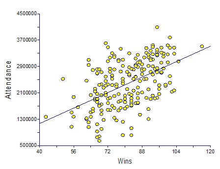
Team Wins in Current Year (Wins)

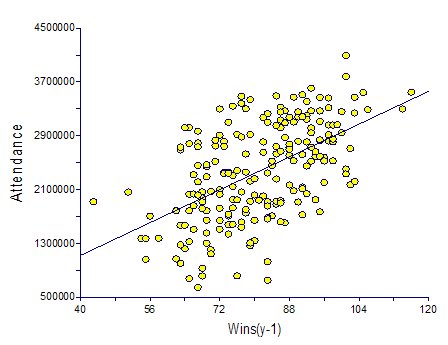
In a straightforward fashion, I included team wins in the current year as a potential predictor of team attendance.

Team Wins in the Previous Year (Wins(y-1))

My previous model, as well as the work by Baseball Prospectus, found that previous year win totals were even more important predictors of team attendance than current year totals. I opted to only consider the previous year's wins. While I could have considered previous years' totals, my previous model found that previous-year totals were just as good as '02 through '05 win totals. Furthermore, using '99-'05 data only gave me 7 seasons worth of data. Increasing the number of previous season win totals I used would have required me to either drop Arizona and Tampa Bay from my dataset or scale back the total number of seasons in my model. I didn't want to do either. Finally, there was another variable available to account for past historical success (or lack thereof):

Playoff Appearances in the Past 10 years (Playoffs)

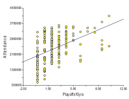
Here I simply summed, for each year, the number of playoff appearances--by winning the division or wildcard--that had occurred in the previous 10 seasons.

Quality of Stadium (Stadium)

Some teams, like the Minnesota Twins or the New York Mets, have rather lousy stadiums. By comparison, 16 ballclubs have built new parks since the White Sox opened the second Comisky Park in 1991. These new parks, which are almost all gorgeous places to watch a ballgame, have resulted in far more enjoyable experiences for fans. MLB clubs claim they increase attendance over the long term. Therefore, I wanted to try to account for this in the model.

Simply including the time since each ballpark was built didn't seem to work, as many old parks--Wrigley, Fenway, Dodgers Stadium, etc--are still fine places to watch a game. Instead, I sought out a mechanism of rating each ballpark. My solution was to use Brian Merzback's Ballpark Review ratings. While it's not as ideal as I'd like, Brian has visited all but one existing major league park, as well as many of the ones that were phased out over this past decade. His reviews seem reasonable and well justified, and I'm pretty much in agreement with him on the 7 or so MLB parks that I've attended. I converted his letter grade +/- system into a 1-13 ranking, with 1 being best and 13 being worst. I had to supplement his ratings with those for the five stadiums that he did not report grades as follows: Bank One Ballpark (B+ based on personal experience, comparing it to GAB and PNC park), the Astrodome (C; might be generous?), Qualcomm Stadium (C; a wild guess), Kingdome (D; based on negative reports I've seen), and Candlestick park (C; based on climate more than anything).

The effect of a new stadium (Honeymoon)

During some initial runs of this model, I found that the most common positive outliers were for teams in the year they open a new ballpark. To account for this, I included a binary variable, Honeymoon, for the first year after a team opens a new park. While this positive effect may remain for years after a new park opens, this simple variable eliminated all of my severe outliers.

Model Selection

If you're keeping score, that is 8 total variables that I am using to explain 7 years of attendance ratings. Several of these variables are sure to be correlated with one another (especially MSAPop and splitMSApop), and one should always be mindful of overloading a model with variables and artificially increasing your R^2. Therefore, I employed used an all-possible subset selection approach to choose the best available model.

After considering all available models (details on how this done are happily given via e-mail or in the comments…didn't want to fuss up this post with those details, as this post is long enough already!), I selected this model moving forward (variables roughly ordered by importance):

Attendance = -117,887*Stadium + 16,297*Wins(y-1) + 13,331*Wins + 513,777*Honeymoon + 496,434*log(splitMSApop) + -2,736,589

This model explains ~61% of variation in attendance rates (adjusted Rsquared=0.5961) from '99-'05. All variables were highly significant (P less than 0.003 for all variables), there were no significant outliers, and there were no signs of heterogeneous variance or deviations from normality. Let's walk through each of these variables:

Stadium: The coefficient on Stadium indicates that for each increment along Merzback's ballpark rating scale, teams gain roughly 120,000 in attendance each year. To put this in perspective, the model predicts that the Metrodome, which got a D-, would pull 1,414,644 fewer fans each year than Wrigley Field, which got an A+. If we assume ~$25 per fan that comes through the gate, that's a difference upwards of $35 million a year! That's a staggering difference. While these numbers are highly contingent on the reliability of Merzback's ratings, this was perhaps the most important factor in the model. Ballpark quality clearly does have a tremendous influence on the revenue a ballclub can gather from attendance.



Wins and Wins(y-1): In both the Baseball Prospectus chapter, as well as my previous article, wins from the previous season seem to be more important that wins in the current season for determining attendance. A win in the current season should increase attendance by 13,000 people, but should also increase attendance by 16,000 in the following season. Let's look at how this should affect influence attendance for the Reds vs. the Cardinals. The Reds won 76 games in '04 and 73 games in '05, whereas the Cardinals won 105 games in '04 and 100 games in '05. Therefore, the Reds would be expected to have drawn (105-76)*16,297 + (100-73)*13,331 = 472,613 + 359,937 = 832,550 fewer fans last year than the Cardinals. At ~$25/fan, that's a difference of roughly $20 million last year. Again, a staggering difference.





Honeymoon: In the year that a team opens in a new stadium, clubs can be expected to draw roughly 500,000 more fans than usual. While this effect does not seem to disappear entirely by the second year, it's dramatically weaker in subsequent years.

MSA Population: In terms of the explanatory power of the model, there was virtually no difference between using the straight MSA-Population values vs. the split MSA Population values, which divided MSA Populations in half for teams in two-market cities. The R-square for the straight model was 0.6051, while the R-square for the split-model was 0.6057 (all other variables were held constant). Furthermore, the coefficient estimates were very similar for both models. Finally, the residuals showed very few differences in terms of the relative rankings of the different teams. The biggest effect I saw was that the White Sox and A's, which had the worst fans (based on residuals) in both models, were further from the pack with the straight MSApop data. The splitMSApop data made for a more uniform distribution. Therefore, I decided to use the splitMSApop data. In all honesty, it doesn't seem to make that much difference.



To look at the variables that weren't selected:

Year: Adding year to the model above resulted in a slight drop in the fit of the model (adjusted R2=0.5942), and it was not at all significant (t=-0.26, P=0.796). A graph revealed almost no visible change in attendance over the years considered in this study.

Playoffs:Adding playoffs to the model did make for a very slight improvement in the fit of the model (adjusted R2 = 0.6004). However, the effect was not significant (t=1.79, P=0.0743). It's admittedly a bit borderline, but given the strength of the other effects, I decided not to include it. It's primary effect, looking at the residuals, was to penalize teams like the Yankees and the Braves in the team residual rankings. This might be appropriate, but I would prefer to keep as many degrees of freedom as I can in the model so that the coefficient estimates are as powerful as possible. It is fairly well correlated with the win variables, and therefore the pattern you see in the graph below is at least represented by the win total data.

Relative Team Attendance

My whole motivation in trying to build a model of team attendance was to take a look at the residuals. The residuals are the differences, in terms of the number of fans, between the actual team attendance and the team attendance predicted by the model. Teams with outstanding fans should come to the ballpark at a higher rate than predicted by this model, while teams with the worst fans should come to the ballpark at a lower rate than predicted by this model. Here is the list of teams and their average residual (mean across 7 years) from this model. The scatterplot on the right reflects the data on the left, with random scatter along the x-axis to make the team names legible):

Team Residual STL 596,368 BAL 573,984 SDP 477,570 COL 472,369 LAD 439,802 SEA 301,698 NYY 282,019 ARI 260,564 MIN 210,327 NYM 151,351 SFG 124,332 CHC 120,932 CLE 105,477 CIN 104,409 MIL 101,225 TEX 40,146 PHI 37,342 TOR -21,309 HOU -57,139 TBD -145,038 DET -170,645 ANA -182,081 ATL -234,519 PIT -284,219 KCR -369,626 WSN -418,037 BOS -542,911 FLA -634,862 CHW -639,697 OAK -699,831

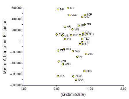As in my earlier attempts, St. Louis fans were the best, with an average of 596,368 fans above what the model would predict. However, the gap has closed considerably. Baltimore, even after accounting for the gorgeous Camden Yards, drew at the second highest relative rate, with Padres, Rockies, and Dodger fans also showing up at well above predicted rates. The Athletics, White Sox, and Marlins came up the worst, drawing more than 600,000 fewer fans each year than the model would have predicted.

The Reds came in just above average, drawing roughly 100,000 more fans, on average, than predicted. Here are the individual years and their respective residuals:
The Reds' best year attendance-wise during that period was 2000, the year following the exciting 1999 season that came one win against the Mets away from entering the playoffs. The model predicted an increase in attendance that year of ~200,000 fans relative to '99, but Reds fans showed up in droves--400,000 more fans than expected!, resulting in the best total attendance during the 7-year period (2,577,371). This was, in fact, more than 200,000 more fans than showed up in '03 for the opening of Great American Ballpark (2,355,259). This relatively poor turnout resulted in the worst Reds residual showing up in 2003, 270,000+ fans fewer than expected in an inaugural season. The moral of the story? Reds fans like winners more than shiny ballparks. Castellini should take note!

Critiques

While I do feel that this work is sound, there are some clear critiques one might offer against it. Here are two, along with some justifications for them:

1. The most obvious problem to a statistics-oriented person is that I've violated assumptions of independence. I treated each year of each team as an independent data point, and clearly that is not an appropriate assumption. The appropriate mechanism for dealing with this is to include the team as a factor in the model. This process assigns a binary variable to all but one team, the last team being identified when all those variables read "0." The problem with doing this, and the reason I did not do it, is that these binary variables capture the differences unique to each team. It was precisely these differences that I wanted to quantify as a measure of fan interest. I could look at coefficients in front of each binary variable, but I would not get to see the coefficient for whichever team did not have a binary variable. Furthermore, these team variables would confound with my measures of metropolitan population and stadium quality, which were relatively constant within each city. … So it made sense to me to do it the way I did.

But I'm sure all of my former stats teachers are groaning right now. In an attempt to placate them, I did go ahead and run the model "correctly" to see how much of an effect my assumption violation had on the coefficients of the model. Here they are:

Variable	Coefficent from my "bad" model	Coefficient from the "right" model
Intercept	-2,736,589	-164,622,313
log(splitMSApop)	496,434	2,414,243
win(y-1)	16,297	14,811
win	13,331	13,552
stadium	-117,887	-46,473
honeymoon	513,777	539,525

As you can see, there was an effect, particularly for splitMSApop and stadium quality, but this is not surprising. Each team tends to have a fairly steady city population (except Montreal/Washington), and most teams did not switch ballparks from '99-'05. Therefore, including a variable for team pulled some of the variance away from these variables and thus changed the coefficient estimates.

Fortunately, the other three variables--win, win(y-1), and honeymoon--were relatively unaffected. Therefore, I feel good about my decision to use the model I did. I'm sure some people may disagree, but this is just for fun anyway. :)

2. I used relative attendance as my measure of fan interest. While this usually works fine, it can become a problem in a few circumstances. This was particularly notable for the Boston Red Sox. I think most people would expect their fans to be at least as supportive of their team as those of the Yankees, if not more so. However, Fenway Park has the smallest capacity of any major league park at 33,871, which puts their maximum annual attendance (assuming 81 games) at 2,743,551. The Red Sox have pulled just about this number each year in this study, and yet they are pegged as pulling roughly 500,000 fewer fans than expected by the model. I'm certain that if their ballpark had a higher capacity, they'd perform much better in this analysis.

A solution to this would be to look at total revenue for the teams, rather than just attendance. I have yet to come up with these data, although I hear that Forbes magazine publishes annual financial reports on MLB teams. In future work, I may take those figures and use them in lieu of attendance to see how things change.

For now, however, I'm going to leave this where it is. This has been a fun exercise, but I've taken it as far as I really care to for now. If folks are interested in fiddling more with the numbers, here is my excel spreadsheet (most stats were done in SAS or NCSS). All I ask is that you provide credit should you use it in your own projects. Thanks, JinAZ